Dynamic Model of a

Horse Gallop in 2D

Eddy Boxerman

Introduction

I did this project for Michiel van de Panne's animation course at UBC in the term of Winter 2002.

The goal of the project was to model the dynamics (forces, torques) of a horse gallop on computer, and to determine a stable control strategy for a sustained gallop. The scope of the simulation was restricted to 2D, although in principle the method expands naturally to 3D.

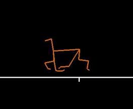
An animation is worth a thousand words. The following two animations demonstrate the results of the project.

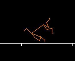A few cycles of a stable gallop	A gallop becoming unstable

Note: although all renderings are of simple skeleton models, more complex inertial body properties were used in the simulation.

Motivation and Related Work

Much can be learned from studying the graceful motion of animals. The topic of animal motion control touches upon such disciplines as control theory, biomechanics, robotics, artificial intelligence, and computer animation. A good overview of the problem, from a computer science perspective, can be found in [6].

Traditionally, computer animation relies on techniques such as key framing and motion capture. However, the former can be tedious and time consuming while the latter is difficult to generalize to differing models, motions and environments. Dynamic simulation has the potential to produce realistic animations in a more automated fashion.

Dynamic simulations of animals gaits (including horses) such as walking and trotting have been done [7]. In fact, as an intermediate step in this project, I simulated a horse trot. However, the trot is a simpler (symmetric along the sagittal plane) and more stable gait than the gallop. To the best of my knowledge, a dynamic simulation of a horse gallop had not yet been accomplished.

Materials

This section describes the data and tools used for the simulation.

Model

The horse was modeled using a 2D articulated figure.

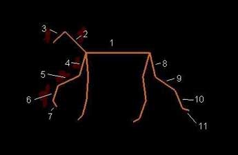Visualization of horse model used in simulation (segment numbers identified in table below)

Muscle actions are simply modeled as joint torques over time. Model dimensions, inertial properties, and target motion data were gathered from various sources. The model was then simulated on computer in an attempt to achieve a stable control strategy for a sustained gallop.

Dimensions and Inertial Properties of Model

Inertial properties of the various body segments were extracted from [1]. Slight modifications were made to conform to the model being used. The following table contains the inertial parameters that were used in the simulations.

Note: Center of gravity is the distance of a segment's COG (along its axis) as measured from its parent link. The Trunk segment's COG is directly at its midpoint.

Gait Poses

The first successful sequential photographs of rapidly moving objects were taken by Muybridge [2]. A main focus of his work was horse gaits. A twelve frame sequence of a horse gallop (Plate 67) was used to define the target poses of the simulation.

A horse gallop stride in 12 phases (taken from [2])

Body segment lengths and joint angles were extracted directly from the photographs with a trusty ruler and protractor. While this does not yield precise values, it suffices for this purpose. In fact, since a reasonably stable gallop was produced, it demonstrates the technique's power to overcome relatively poor initial data.

The following animation displays a rendering of the extracted data. Note that this is not the result of a physical simulation, but merely a projection of the poses against a ground plane (notice how the torso remains perfectly horizontal).

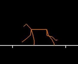Visualization of pose data extracted from [2]

The measured joint angles can also be found in the following (tab delimited text) file.

Dynamics Simulator

To simulate the system dynamics, I employed Michiel van de Panne's 2D dynamics simulator. First a "dynamics compiler" - given a description of a 2D articulated figure - produces a symbolic description of the equations of motion in the form of a 'C' procedure. The procedure is then linked with a dynamics engine which, when executed, calculates the system state (forces, torques, rectilinear and angular positions and velocities) over time. The engine simulates ground reaction forces using a penalty based method.

For the purposes of this project, I expanded the simulator to accept additional simulation parameters such as: target poses for the articulated figure, joint stiffnesses, etc. For the purposes of running test suites as well as monitoring and organizing results, I wrote several perl scripts. I also wrote a C++/OpenGL utility for rendering and capturing the animations.

Methods

In the context of this project, modeling a stable gallop consists of finding the correct combination of parameters for the simulation. The problem then becomes one of searching for a solution in some high dimensional space. To this end many simulations were executed with varying parameters, guided by an optimization scheme and rejection criteria.

Simulation Parameters

The following parameters are used in the horse simulation. The Min and Max columns identify the ranges of values that are legal (may be attempted) for each parameter.

This gives a total of 311 parameters, a high dimensional space to search. In order to reduce this number, I made the following assumptions and adjustments:

The search algorithm used is similar in nature to that found in [6] with a few adaptations to the problem at hand. It begins with a global search of the parameter space, followed by local searches of promising regions that were discovered by the global search. It is arguably related to such algorithms as simulated annealing and greedy optimization. The pseudo code is as follows:

• Simulation Time <- 2.0 seconds
• Randomly generate parameters (use full ranges) and evaluate via simulation for 1000 sets.For any simulation that is not rejected, add that set of parameters to the successful trial database
• Perturbation Factor <- 0.3
• Repeat until trials converge (or you're fed up waiting)

  • For each of the 10 best trials
    • Perturb the parameter set of the given trial and evaluate via simulation. If it is not rejected and the optimization metric is higher than the original's, update the parameter set and continue searching.
  • Simulation Time = Simulation Time * 1.5
  • Perturbation Factor = Perturbation Factor / 3
• Output best parameter sets

A few terms and details require explanation:

• Rejected Simulation: this refers to any simulation in which the horse model violates a rejection criteria. These are defined by the Joint Limit, Torso Limit, COG Limit and Joint Velocity Limit parameters defined above. For instance, if the model violates the Torso (angle) limit, it is probably about to flip over - definitely an unsuccessful gallop. More subtle is the Joint Limit criteria: if at any time any joint deviates from its target angle by more than a threshold value, the gait is rejected. Before implementing this restriction, I observed some interesting and successful (relatively fast) gaits, but they did not resemble a horse gallop! By adding this restriction, only gaits that are similar to the gallop are accepted.
• Perturbation Factor: This value controls the percentage of the Min / Max range that is explored through randomization. For instance, when Perturbation Factor = 0.05, the perturbed parameters will only deviate from the current set's by up to 5% of the ranges as defined in the parameter table. It is initialized to 0.3 once the algorithm begins its local searches. As more and more successful parameter sets are found, this value decreases, shrinking the perturbation ranges and refining the local search.
• Simulation Time: Finding a long-term stable gait is a delicate matter [5]. It is much easier to find one that is stable for a short period of time. Hence, the algorithm begins its global search for gaits that are stable for at least 2 seconds. At each stage of the search, the Simulation Time is increased to ensure that the gaits become stable for longer periods of time - ideally forever.
• Optimization Metric: the criteria used to judge a (non-rejected) parameter set is simply distance traveled. This was chosen over velocity so that parameter sets that were run for different Simulation Times can be compared against one another; ie. when comparing a fast but unstable gait to a slower but longer-term stable gait, the more stable gait should be chosen.

Results

Overall, the results obtained from the approach described were good. Some animations are provided.

Over several runs of the search algorithm, the most successful gallop found was stable for 22.77 seconds of simulation time, or for approximately 86 gait cycles. The parameter set for this simulation can be found in the following file. For convenience, some interesting values are presented in the following table:

In general, production of stable gaits lasting up to 10 seconds was quite common. No indefinitely stable gait was found. The question remains open as to whether an indefinitely stable, open-loop gallop exists.

As for simulation performance, it runs in approximately real-time. ie. it requires about 10 seconds to execute a simulation that models 10 seconds of simulation time. Typically, gaits that were stable for 2-3 seconds could be found within a few minutes of searching; and gaits that were stable for 10 seconds required about 1-2 hours of searching.

Analysis

Encouragingly, various properties of the simulated gallop that were not explicitly controlled were found to conform quite closely with a real gallop:

An additional metric which would prove useful for analysis is foot-fall timing of the simulated gaits; which could provide quantitative evidence that the simulated gallop has the same phase characteristics as a real gallop. Unfortunately time did not permit this.

An aspect that should be reconsidered is that all initial angular joint velocities were set to zero for the simulations. However, the initial state of the system should in fact represent a point in the steady state of a horse galloping. In retrospect, appropriate initial velocity ranges should have been chosen and these parameters should have been randomized as well. While this would have increased the number of search parameters by 18, perhaps these too could have been postponed until later phases of the search (as the poses themselves were).

Conclusion and Future Work

The results of this project are encouraging and lay a solid foundation to work from. The technique in theory could be applied to any creature-gait combination that is symmetric in the sagittal plane. Other interesting animal subjects in Muybridge's book include baboons, gazelles, dogs, kangaroos and ostriches!

The technique applied here should generalize naturally to three dimensions. This entails more complicated simulation techniques and higher dimensional spaces, but the approach and algorithm should remain essentially the same.

As already mentioned, initial angular joint velocities should not be assumed to equal zero. This in itself may be causing the initially successful gaits not to converge to stable long-term gaits.

Currently, the optimization criteria used to judge the success of a gait - and to choose a parameter set to locally search - is based on distance traveled. Another alternative is to consider energy expenditure; or distance traveled. per energy expended. This may prove useful since it is generally accepted that animal gaits use energy efficiently.

Of course, closing the loop could provide an indefinitely stable gait. Various techniques that decouple or linearize the complexity of this problem can be found in [3] and [4]. The work here involves finding a few key simulation states to monitor and a few control parameters that could be adjusted "in-simulation" to compensate for the state divergence. A good candidate for states to monitor may be foot-fall timings, which could be compared to actual gallop timings. Indirect control over the timings may be achieved via modifying the model's compliance (Joint KS parameters) temporarily, or by adjusting the interpolation parameter accordingly (ie. if the target pose is in a post foot-fall condition, but the foot-fall in the simulation has not yet occurred, the interpolating parameter could be "slowed down" to wait for the foot-fall to occur).

Fleshing out of the skeleton-rendering would yield more attractive results of course.

Acknowledgments

I'd like to thank Michiel van de Panne for his help and suggestions during this project; as well as for allowing me to use his simulator.

References

[1] Buchner, H.H.F., Savelberg, H.H.C.M., Schamhardt, H.C. and Barneveld A. (1997) Inertial Properties of Dutch Warmblood Horses. JOURNAL OF BIOMECHANICS 30(6) pp 653-658

[2] Muybridge, E.J. (1887). Animal Locomotion.

[3] Laszlo, J. F., van de Panne, M., Fiume, E. (1996) Limit Cycle Control and its Application to the Animation of Balancing and Walking, SIGGRAPH 96 Conference Proceedings (ACM Computer Graphics), 155-162.

[4] Playter, R. (2000) Physics-based simulations of running using motion capture. SIGGRAPH 2000 Course Notes, Course #33

[5] van de Panne, M. Lamouret, A. (1995) Guided Optimization for Balanced Locomotion. Computer Animation and Simulation '95 -- Proceedings of the 6th Eurographics Workshop on Simulation and Animation, Springer Verlag. Maastricht, Netherlands, 165-177.

[6] van de Panne, M. (2000) Control for Simulated Human and Animal Motion. IFAC Annual Reviews in Control 2000, 24(1), Elsevier Science Ltd., 189-199.

[7] Villanova, J., Guinot, J-C., Neveu, P., Gasc, J-P. (2000) Quadrupedal Mammal Locomotion Dynamics 2D Model. Proceedings of the 2000 IEEE/RSJ International Conference on Intelligent Robots and Systems.